Introduction
The goal of this course is to become familiar with collecting data in the field to use for geospatial analysis, and this lab works toward achieving that initiative by working with and learning about yet another data collection mobile application. In today's lab, ArcCollector for iPhone was the application of choice. This application (also available for android devices) allows users to crowdsource data with predefined attribute tables in real time. The data collected in this lab will be used to create a microclimate map of UW - Eau Claire's campus (see Results section).
Study Area
The study area for this lab consists of the UW - Eau Claire campus divided into seven smaller study areas (see figure 1). These areas will be covered by two students each and the goal is to get 20 points collected for each student in each area.
Figure 1: Map of study area.
Methods
The first step to completing this lab is to download the app on a mobile device. Once the app is downloaded, sign-in to ArcGIS Online through the app. Navigate to the class group form (figure 2) and a basemap containing the various group areas for collection, as well as collected points, are visible (figure 3).
Figure 2: Navigate to the correct class group.
Figure 3: View group zones and collected points in ArcCollector app.
For this lab, two students were assigned to each group study area (I was in group study area one). Once each group gets to their respective study areas, tap the + button in the app, and the data collection can begin. The data being collected is as follows:
Group study area (GRP)
Temperature (TP)
Dew Point (DP)
Wind Chill (WC)
Wind Speed (WS)
Wind Direction (WD)
Notes
Time (of collection)
The form to collect this data looks like that of figure 4.
Figure 4: Data collection form in ArcCollector app.
After the data has been collected in the ArcCollector app (see figure 3), navigate to ArcGIS Online at a desktop computer. Log in with the appropriate credentials and a map with the collected points will be available for use under My Content. Open the map details and click Open in ArcGIS Desktop (shown in figure 5).
Figure 5: Open in ArcGIS Desktop.
From there, the data points, all attributes collected , group study areas, and basemaps are available to create a series of microclimate maps.
Results
The two resulting maps show 1. Wind speed and direction and 2. Temperature of various points collected by the students of this class. Of course, there was some error in data entry, however, for the most part the data collected was good data. Personally, I accidentally entered in wrong data and had to go back and change it before moving on to the next point, but error can occur easily when using this app if the collector isn't careful.
Figure 6: Wind speed and direction map.
In this map (figure 6), the wind speed was represented as a graduated symbol. This means that the faster the wind speed, the bigger the symbol. The arrows also show what direction the wind was blowing.
Figure 7: Temperature map.
In this map (figure 7), temperature was symbolized as a graduated colors. Green was colder and red was warmer.
Discussion
Looking at the results first, the wind speed and direction map was really interesting. I've never used the rotation symbology feature before but it's cool that from the data (wind speed and direction) a map such as this could be made, all because my classmates and I collected the information. The temperature map was also intriguing. Seeing as the study area only covers less than a square mile, one would think the temperature wouldn't vary a whole lot. With the data collected, however, there was over a 20° difference in some places on campus.
Overall, I thought the ArcCollector app was an efficient and easy-to-use data collection app. The real-time data point map was a cool feature- especially when we were out in the field, it helped my partner and I to keep up with the rate at which other students were collecting their data. From an administrative standpoint, this feature could be useful in ensuring that students/employees/etc are indeed collecting data. Other than a few incorrect entries, the data was fairly consistent, so symbolizing and classifying the data was easy to do.
Introduction
As far as accessible platforms for working with GIS, mobile apps are quickly gaining popularity. For this lab, Survey 123 was used; an ESRI application that allow the user to create a survey, collect data (through mobile devices), and publish that data as web apps, maps, and other platforms. An ESRI Online lesson was used to familiarize the students with how this platform is used (see Methods section) in the scenario that data was being collected for an emergency preparedness survey.
Methods
The first step to collecting survey data is to create the survey. To do this, go to the Survey 123 website and sign in with either an Enterprise account or an ESRI account. Once signed in, click the "Create New Survey" button (figure 1).
Figure 1: Create New Survey button (highlighted at top).
Next, give the survey a Name, Tags, and Summary. The user can choose a thumbnail for their survey as well, however this is optional. Once the information is completely filled-out, click Create (figure 2).
Figure 2: Create New Survey information window.
Now that the survey has been created, questions must be added to collect information from the end user. The questions used in this survey are:
Q1: Date
"Survey completion date:"
Required*
Q2: Single line text
"Participant Name:"
Required*
Q3: Single line text
"Participant Location:"
Hint - "e.g., address, street name, or nearest cross streets"
Required*
Q4: Geopoint
"Locate your residence on the map:"
Hint - "Note: If you would prefer to not locate your home, please use the nearest intersection/ cross streets."
Use "Street" ESRI basemap
Q5: Single choice question
"What type of residence do you live in?"
Options:
Single family (house)
Multi-family (apartment, condo)
Q6: Number
"How many levels does your home have?"
Hint - "include basement as separate level (if applicable)"
Set Rule for Q5:
Click icon shown in Figure 3
If the answer is Single Family (house), show the question How many levels does your home have?
Figure 3: Set Rule icon.
Q7: Number
"Approximately what year was your residence built?"
Validation - must be an integer
Q8: Picture
"Picture of your residence"
Hint - "This will help assess the building materials and structural integrity. For security reasons, please do not share pictures with personally identifiable elements such as house numbers or car license plates."
Q9: Number
"How many people live in your home?"
Validation - must be an integer
Q10: Multiple choice
"What are the age ranges of the people who live in your household?"
Hint - "check all that apply"
Set choices to:
0 - 5 years old
6 - 17 years old
18 - 60 years old
> 60 years old
Horizontal Layout
Q11: Single choice
"Safety Check 1: Are the televisions in the home secured?"
Hint - "e.g., secured to where they're located, such as the cabinet, table, or wall?"
Set choices to:
Yes
No
Q12 and Q14: Drop down
"How are they secured?"
Set choices to:
Locks
Pad
Straps
Velcro
Set rule(s) for Q11 and Q13 to:
If the answer is Yes, show the question How are they secured?
For questions 13, 15-19, 21, and 23, repeat the same format as Q11 (starting with "Safety Check #" and Yes/No answer). Here are the following "Safety check" questions:
Q13: "Are computers in the home secured?"
Hint - "e.g., secured to where they're located, such as the desk or table?"
Q15: "Are bookcases secured to the walls?"
Q16: "Are large cabinets secured to the walls?"
Q17: "Are any objects placed above sofas and/or beds?"
Hint - "e.g., framed pictures, mirrors."
Q18: "Are all exits (doorways to outside) clear of obstruction?
Q19: "Are functioning smoke alarms present in each room?"
Q20: Number
"When were they last tested to be in working order?"
Hint - "estimate number of days"
Q21: "Are there fire extinguishers in the home?"
Q22: Number
"How many extinguisher units?"
Q23: "Verify there are no overcharge plugs in the home."
Hint - "e.g., no multi-plugs plugged into a multi-plug."
Q24: Single choice
"Is someone in the household trained in First-Aid?"
Set choices to:
Yes
No
Q25: Multiple choice
"Select items in your home that could be used in case of an emergency response
Hint - "check all that apply"
Set choices to:
Axe
Batteries
Blowtorch
First-aid kit
Flashlight, candles, matches
HAM Radio or AM/FM radio
Handheld radios
Ladder
Portable generator
Satellite phone
Saw
Shovel
Stockpile of food and water for 7 days
Tent
Town/city map
Wheelbarrow
Q26: Single choice
"Do you have an up to date emergency contact list or phone tree?"
Set choices to:
Yes
No
Q27: Single choice
"Do you have a current evacuation plan?"
Set choices to:
Yes
No
Q28: Single choice
"Do you have a local neighborhood or community disaster plan?"
Set choices to:
Yes
No
Q29: Multiline text
"Additional comments:"
Hint - "please list other resource items that could be useful in an emergency"
To do this, click Add Questions from the Design window (figure 4). There are many different question types to choose from.
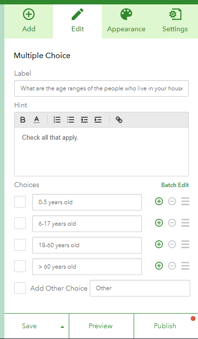
Figure 4: Adding a multiple choice question from the Add Questions tab of the Design window.
When one is selected, the survey author can edit the settings of the question. In Figure 5, the label is set to the question "What are the age ranges of the people who live in your house?", the hint is set to "Check all that apply.", and four different options are given for the question choices.
Figure 5: Edit question settings.
Once the settings for each question are satisfactory, click Save (bottom left in figure 5) and the question settings are applied to the survey. Once all of the questions are entered into the survey, click Publish (bottom right Figure 5). The survey is made and end-users can access the survey through the Survey 123 mobile app or the website. In order to see how the collected data can be used, ask friends or colleagues to take the survey.
Figure 6: Open Survey 123 app and tap Download Surveys (top right).
Figure 7: Select survey to download.
Figure 8: Complete survey.
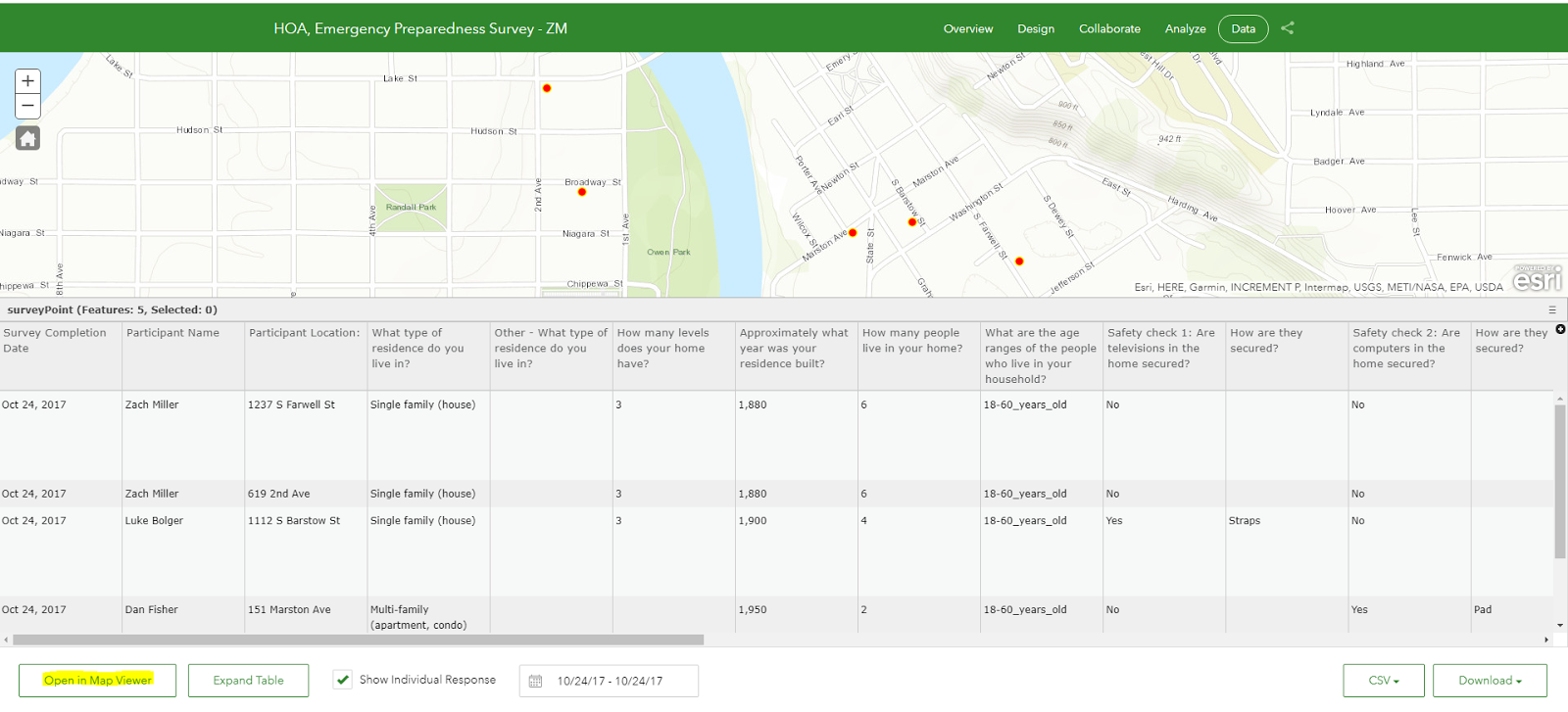
Now that the survey has collected data, go to the Data tab in the survey settings (figure 9).
Figure 9: Data viewer in Survey 123 online.
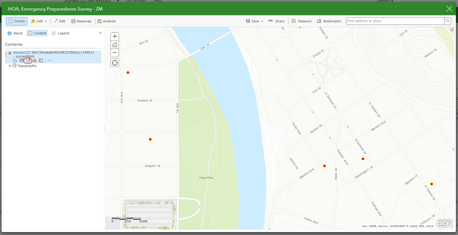
Click Open in Map Viewer (highlighted in Figure 9) and ArcGIS online will open in a new tab with the data collected from the survey shown as points (figure 10).
Figure 10: ArcGIS Online Map Viewer.
From there, adjust symbols (red circle in Figure 10), configure pop-ups, and select theme for a web app to share this data with an organization or the ESRI community (figures 11 and 12).
Figure 11: Configure Attributes (to be shown in pop-up window).
Figure 12: Choose template for new Web App.
The resulting data and web app can now be used to analyze the information collected by this survey.
There were some trends that ensued when analyzing this fake data (I completed 5 surveys with various answers). Some of which include:
All who took the survey were college aged students.
Most who took the survey lived in single family homes.
Most who took the survey did not secure their T.V., computer, or bookshelves.
60% of those who took the survey had an axe, some batteries, and/or a First-aid kit.
*Note: these numbers can be found in the Analyze tab of the online survey viewer.
Discussion
This technology can be extremely useful as smartphones are becoming more accessible. As seen in the Methods section of this lab, it was fairly easy to create and publish this survey- collecting the data was even easier. In a real scenario, the surveyor would just sit back and let end-users input their answers, allowing the app to collect the data. The interoperability between Survey 123 and ArcGIS online makes visualizing the data through a Web App streamline.
Some drawbacks of this technology are that end-users who don't have the app installed on their mobile device might not want to install it and this can affect the data. Potential end-users might not have access to a mobile device and this would also affect the data. These drawbacks are important to consider when disseminating the survey and the surveyor should ensure that their is an online version explicitly available to those who apply to one or both of the concerns mentioned previously.
Overall, I think this is a really cool way to collect geospatial data in a high-quality and aesthetically pleasing platform.
Data Source
"Survey123 For ArcGIS." Survey123, ESRI, survey123.arcgis.com/
Introduction
The purpose of this activity was to practice using the Bad Elf GPS Unit in combination with the Bad Elf app for an iOS device, which, like the previous assignment, will help in the upcoming navigation lab. When it comes to increased accessibility of GIS data and functionality, smartphones and tablets are on the rise. Think about it- apps like Google Maps, Strava, Find My iPhone, et al are quite popular for everyday navigation/directions, tracking a bike ride/run, and other location services. Utilizing this platform to connect with a GPS unit seems rudimentary, but can greatly increase the functionality of this fading technology.
In addition to using the GPS unit in accordance with the iOS app, there are other apps with a variety of functionalities that are compatible with data collected from the Bad Elf technology. These include the following apps:
Collector for ArcGIS - Free
Collect and update data.
Cache maps for offline use.
Attach photos to collected features (like story mapping).
Access to professional-grade GPS receivers.
Feature and places search.
Track log functions.
Survey 123 for ArcGIS - Free
Simple survey form-based software.
Online survey form download and submission functionalites.
Offline survey data collection and form saving capabilities.
GIS4Mobile-X - Free
Offers data collection and synchronization functionalities.
Allows user to connect collected data to account servers or personal servers.
Theodolite HD - $6 pricing with in-app purchase offers
Allows user to capture and geo-tag photographs and videos with saving/caching capabilities.
User is able to overlay geographic data, time, date, and notes in the photo viewer.
Contains map viewer as well which allows user to view features like roads, trails, et al.
App contains reference angle, navigation calculator, data logging, and .KML export functionalities as well.
Offers in-app upgrades such as "team tracking" which allows up to 20 users to collect data for the same project all at once.
Gaia GPS - Free, Member level ($10/year), and Premium member level ($30/year)
Offers downloadable access to both historic and modern hiking, hunting, off-roading, and otherwise trail-blazing navigation maps.
Allows users to track, sync, back up, and share waypoint data collected.
Also has geo-tagging photograph functionality.
Gelileo Offline Maps - $4 pricing
Allows user to download, search for, and use maps offline.
Allows user to search for maps offline.
Allows user to track, sync, backup, and share data in app.
Contains bookmarking functionalities and map support.
Fog of World - $5 pricing
Allows user to visualize where they have and haven't been in the world.
Tracks and displays where the user has been.
Allows user to sync and share track log data.
Creates statistics based on user's travel experiences.
Methods
For this lab, students were asked to connect a Bad Elf GPS unit to their iOS device to collect a track log of a walk around campus. This track log feature will be used to track student groups when they navigate their way through the upcoming priory navigation lab. The devices pair through Bluetooth and the iOS app collects the user's path from when they push the Track button at the start of their data collection and again to stop their data collection (figure 1).
Figure 1: Bad Elf GPS Pro+ GPS unit.
After the students completed their walk and stopped tracking their route, the data was available for viewing in the iOS app. The data collected included the tracked path superimposed on a satellite imagery basemap, as well as a speed, altitude, and distance tab conatining averages, charts and distances (figures 2, 3, and 4). The green pin was where the track log was started and the red pin was where the track log was stopped.
Figure 2: iOS user interface with speed tab and resulting data shown.
Figure 3: iOS user interface with altitude tab and resulting data shown.
Figure 4: iOS user interface with distance tab and resulting data shown.
From there, the path data was able to be shared through e-mail or for use in other apps as a .KML file. This was done to create the map shown in figure 7 (see Results section).
The .KML was sent from the iOS app to email. From there, the .KML file was downloaded and brought into ArcMap using the KML to Layer tool (figure 6).
Figure 6: KML to Layer tool window.
Results
Figure 7: Resulting map.
Discussion
Overall, I found the functionality and easily operable application to have real-world benefits. Whether the app is used for research or for logging where you walk, run, bike, etc, this app offers access to geographic information to anyone with an iOS device.
One of the things I really like about this app is the ability to export the resulting data to other useful GIS, recreation, or travel apps, as well as desktop applications. Another nice feature of this app was that the user can collect data offline-which seemed to be a common theme among the other mobile apps discussed in the Introduction section.
There were a few downsides to this app as well. One of which was the accuracy of the track log, in figure 7, it is clear to see that some areas of the path aren't fully in accordance with the path I actually walked. For instance, the map shows that I crossed the river and came back Another issue I had with the app was its floating placement in Google Earth Pro (GEP). The polyline was not mapped on the ground in GEP, but rather floating above the surface. This can be problematic for users who only have access to this program or other programs that could produce this error.
For this assignment, the goal was to produce two maps of an area *three miles* south of the UW - Eau Claire campus; the Priory residence hall. In a later lab, student groups will have to navigate their way through the Priory's forest using only the GPS points of the route and their maps.
To start with a bit of background knowledge on coordinate systems was an important part of creating these maps (see Results section). Coordinate systems are a common tool used for navigation in coordination with others such as Global Positioning System (GPS) units. Since the Earth is 3-D and maps are usually 2-D, such as the ones created for this assignment, these coordinate systems endure distortion when making the transformation- the projected coordinate system attempts to minimize that distortion. The two coordinate systems used for these maps are the unprojected geographic coordinate system (GCS), and a projected coordinate system (PCS), the Universal Transverse Mercator (UTM).
Figure 1: Geographic Coordinate System (Environmental Research Institute, 2016).
The GCS was the coordinate system used to make the first map for this assignment. This coordinate system is based on degrees of latitude and longitude originating from the center of the Earth (see figure 1). The intersection of the prime meridian and equator serves as the central axis for this system. The degrees can be written in decimal degrees or degrees minutes seconds, both of which will be used in the future navigation lab in coordination with GPS coordinates.
The PCS used to make the second map for this assignment was the UTM. This PCS is a cylindrical projection that divides the Earth into 60 zones (figures 2 and 3). On a local level (mapping within one zone), this projection minimizes distortion of surface features better than the GCS.
Methods
Once the two coordinate systems used for this lab were conceptualized, those concepts were used to make two navigation maps in ArcMap. For this assignment, the students were given a few different data files to choose from: a USGS topographic map, some aerial imagery covering the land surrounding the Priory, some LiDAR digital elevation models (DEMs), a two foot contour line shapefile, and the navigation boundary. Since the class will be traversing some varying terrain, I felt it was important to include the layers that would show me the variations in terrain, so I chose to use the DEMs and the USGS topographic map for a layered hillshade.
To produce these maps, I started by bringing in the Navigation Boundary layer, USGS Topographic Map raster, and the LiDAR DEM rasters to a blank ArcMap document (figure 4).
Figure 4: Layers used to produce both maps.
Once this was done, ensuring that the coordinate systems of each layer were either the GCS or UTM coordinate systems uniformly was the next step. I began with the UTM map. To do this, the coordinate system was established in the data frame properties, then each layer was projected to the correct coordinate system (if it wasn't already).
First, right-click Layers in the table of contents window and click on Properties. This will take you to the data frame properties window. From there click on the Coordinate System tab and ensure that the coordinate system is checked to NAD_1983_UTM_Zone_15N.
Next, right click on each of the layers shown in Figure 4 and go to their Layer Properties to determine if they need to be projected. This information can be found in the Source tab (figure 5).
Figure 5: Layer Properties window displaying that the layer is already projected in the correct coordinate system.
If a layer has a different coordinate system than the one highlighted in Figure 5, then it needs to be projected. To do this search for the Project tool (if shapefile) or Project Raster tool (if raster file) in the search window or toolbox window of ArcMap.
Figure 6: Project tool window.
A popup window will open (figure 6). Set the input raster, output raster location and name, and appropriate coordinate system. Do this for all subsequent rasters and shapefiles.
One trick for this is to import the coordinate system from a layer known to have the appropriate coordinate system (figure 7).
Figure 7: Add coordinate system from layer with known coordinate system.
After all of the layers were converted to the same coordinate system, the layered hillshade was created. This was done by first organizing the layers correctly:
First, ensure that the Navigation Boundary layer is listed at the top of the drawing order, then the USGS Topo layer, then the DEM layers.
Next, set the Transparency property of the USGS Topo layer to 70% in the Layer Properties window, under the Display tab (figure 8).
Figure 8: Set transparency of USGS Topo layer.
Then, check the Use hillshade effect box in each of the DEM Layer Properties' (figure 9).
Figure 9: Check the Use hillshade effect box for DEM layer properties.
Upon creating the layered hillshade, the map was made by switching from Data View to Layout View. From there, the following were added to the map:
North arrow
Scale bar
Projection, coordinate system, author, and data source information
Labeled grid
To create the second map using the GCS, just repeat the above steps, but with the GCS instead of the UTM coordinate system.
Results
Figure 10: Navigation map using UTM projection.
Figure 11: Navigation map using GCS.
Discussion
The purpose of these maps are to provide the student with resources that will be used to aid their navigation through the navigation area. While many other students used the 2 ft contour shapefile with the Eau Claire imagery underneath, I felt as though I wouldn't be able to use that information effectively in the field. Knowing a bit about myself and the nature of this activity, I figured really getting a sense of variations in the landscape would help me to be most effective in navigating my way through the upcoming lab. Having once upon a time striven for a geology minor, the spatial recognition of physical landscape and terrain features resonates with me more so than surface features and the busy 2 ft contour lines. Hopefully using the data I did will prove to help me effectively work through this lab.
Looking at the resulting maps (figures 10 and 11), I feel as though the UTM map (figure 10) will be more effective to use instead of the GCS map (figure 11). With the 50 meter scale and less distorted projection of figure 10, it will aide in more accurate navigation than figure 11, which is distorted and has a larger grid scale- creating more room for error.
Introduction
The purpose of this lab was to survey the Litchfield mine site, a mine in the southwestern portion of Eau Claire, by using various unmanned aerial system (more commonly known as UAS) platforms and geographic coordinate collection systems. Using a multitude of devices that ranged from entry-level to survey-grade, the class was able to conceptualize the differences in quality and accuracy between them.
Figure 1: Location of Litchfield Mine Site.
Methods
Upon arriving at the site, the class broke into small groups and walked around the site to set ground control points. Ground control points, or "GCPs", are used in UAS surveying to give the resulting composite imagery a location when mapping. Since the site covers roughly 1,550 acres, it was important to get good coverage of the site with GCPs. Putting GCPs too close together can distort the processed imagery, so the class was sure to spread out their placement. GCPs can be made of many different materials, and for this lab the class used high density polyethylene squares, pictured in figure 2 below.
Figure 2: Collecting GCP coordinates with Topcon HiPer SR GPS.
Once the 16 GCPs were placed throughout the site, the small groups went to each of the GCPs and collected geographic coordinates using several different GPS recievers. These consisted of: Apple Maps for iPhone, Bad Elf GPS Unit, Topcon HiPer HR Survey GPS, and Topcon HiPer SR GPS. When processing the data in a later lab, the differences in accuracy will be assessed.
Figure 3: Field log of BadElf GPS and Apple Maps coordinates.
Figure 4: Hand-drawn field map of GCP locations.
Some field notes were taken to record a "mental map" of where the GCPs were placed and the coordinates of the BadElf GPS unit and Apple Maps (Figures 3 and 4).
After collecting the GCP coordinates, the UAS platforms were flown. The first of which was a DJI Phantom 3 Pro. This UAS is a four blade multi-rotor aircraft and is considered a low-level commercial drone due to its somewhat limited capabilities for mapping, payload, and battery life/flight time. Although this drone is not as powerful as some of the other drones used that day, its still equipped with pre-flight mapping capabilities, smart batteries/return-to-home features, and a 20 megapixel (MP) camera. This flight was a successful one, capturing over 200 images of the site in around 15 minutes.
Figure 5: DJI Phantom 3 Pro
The next UAS platform flown was the Sensefly eBee. This UAS is considered a mid-level commercial fixed wing drone, equipped with standard pre-flight mapping and return-to-home capabilities, real time kinematics, and a 20 MP camera. Since this UAS is a fixed wing, it needed more space to land than the multirotors used during this lab. One interesting feature of this drone is that the propeller stalls when taking a photo, which is supposed to increase the quality of the images taken with this platform.
Figure 6: Sensefly eBee
Unfortunately, this drone malfunctioned and crashed after the remote pilot noticed the lack of stability during flight due to high winds, aborted the mission, and attempted to return the drone to its launch point. The drone was recovered in the Chippewa River due west of the site by using another UAS' perspective to locate it; the DJI Matrice 600 Pro.
The DJI Matrice 600 Pro was the third UAS platform flown. This mid-level commercial, six-blade multi rotor was equipped with standard pre-flight mapping and return-to-home features, real-time kinematics, and a 16 MP GeoSnap Pro camera from Field of View. This wide angle sensor is especially good for remote mapping applications. This flight was a successful one, taking around 10 minutes to fly the site; a shorter amount of time than the Phantom 3.
Figure 7: DJI Matrice 600 Pro (a.k.a. M600 Pro)
The final UAS platform flown was the C-Astral Bramor. This high-level fixed wing drone costs over $70,000 and was equipped with advanced pre-flight planning and return-to-home features, a 24 MP camera, and a parachute landing mechanism. This platform uses a tension-loaded catapult launch that flings the aircraft into the wind, lifting it before engaging the automatic propellers which then raise the drone to its predetermined mission altitude. The planned flight took around 30 minutes, however there was a malfunction with the parachute deploying during landing. The aircraft flew over its designated landing zone and flew straight into the forest on the east side of the site. The drone was recovered and is being replaced by C-Astral free of charge due to a programming error.
Figure 8: C-Astral Bramor
In addition to the UAS flights, a Topcon GT ground station was used to demonstrate how it could be used to calculate volumetric data by collecting survey points on a stockpile at the site. This total station is survey-grade, collecting measurements automatically with less than millimeter accuracy- the most accurate measurement device of the day.
Figure 9: Topcon GT total station.
Discussion Using the different GPS methods for collecting GCP coordinates will hopefully put accuracy of each platform into perspective. With the way technology is progressing nowadays, it was no surprise that each platform was fairly simple to use- each having a minimalist visual interface with icons and buttons to collect coordinates with a simple tap of the screen. There were noticeable pros and cons to each platform, however. For the mounted GPS receivers, the coordinates are stored electronically, and can be uploaded directly to the computer for use, however, these systems are usually quite expensive and less mobile than the BadElf GPS unit or iPhone. In turn, the BadElf GPS and iPhone requires that the user manually log their usually less accurate coordinates, but are also cheaper, usually more accessible, and more mobile than their more sophisticated counterparts. Ultimately, which platform to use is subjective to the project and the resources available to the user.
Watching the various UAVs fly was certainly helpful in understanding the differences of the mapping frontier that is unmanned aerial systems. Though both multi-rotors were successful in their flights, the fixed wings weren't so lucky. Both the eBee, a $30k aircraft, and Bramor, a $70k aircraft, malfunctioned and crashed in the same lab- a rarity I'm sure. It was surprising to me, considering how much these things cost, one would think they would be more reliable. Although the failure of both fixed wings was probably an isolated incident, it just goes to show that the industry is delving into some unknown territory and are still working out some kinks. I must say, it was a huge disappointment to not see either fixed wing perform a proper landing, but that's the way it goes sometimes. On the other hand, both multi-rotors proved to be a more reliable and versatile platforms. Having never personally witnessed a multi-rotor malfunction or crash, they can land in smaller areas than fixed wings and seem to give the user more control over the aircraft. In theory, I do feel as though fixed wings could provide more accurate imagery and data than multi-rotors, but the models I've seen fly tend to require more set-up and have a greater risk of error with characteristics such as belly landings, requiring a large and level path for landing, and less pilot control.
The Topcon GT total station was interesting to learn about as well. When observing the tools used on a construction site, one can expect to see a ground surveyor more times than not. These devices are very impressive in terms of accuracy, and for certain sectors, this is of utmost importance. The platform requires more set-up and time than using a UAV, but again, which tools to use are subjective to the what is needed for the project and if less than millimeter accuracy is necessary, than it would be worth it to use this platform.
Overall, I got a lot out of this lab. Having taken a UAS class last semester, I was familiar with what GCPs were, how GPS receivers were used, and the process of flying unmanned aerial vehicles. In addition to seeing the eBee and Bramor fly for the first time, I was able to expand on and dive deeper into my prior knowledge of UAS and witness how survey ground stations work/why they're still used instead of UAVs. I also witnessed my first UAV crashes as well, something very shocking to me.